Seurat (七) 判断某个细胞群的性质 (一) ——GSEA分析

第一步 读取数据

library(Matrix)
library(Seurat)
library(plyr)
library(dplyr)
library(patchwork)
library(purrr)
 
rm(list = ls())
# 配置数据路径
root_path = "~/zlliu/R_data/TCGA"
 
# 配置结果保存路径
output_path = root_path
if (!file.exists(output_path)){dir.create(output_path)}
 
# 设置工作目录，输出文件将保存在此目录下
setwd(output_path)
getwd()

第一步 得到指定群的差异基因

scRNA[['manual_3']] = ifelse(scRNA[['manual_2']] == "Unkown_10", "Unkown_10", 'others')
Idents(scRNA) <- scRNA[['manual_3']]
all_markers <- FindAllMarkers(scRNA, min.pct = 0.25, logfc.threshold = 0.25)
significant_markers <- subset(all_markers, subset = p_val_adj<0.05)
write.csv(significant_markers, 'manual_2_Markers.csv')
significant_markers <- subset(significant_markers, cluster=="Unkown_10")
rownames(significant_markers) <- gsub("\\.(\\.?\\d*)","",rownames(significant_markers))
fc <- with(significant_markers, mean(abs(avg_log2FC)) + 1*sd(abs(avg_log2FC)))
usignificant_markers <- subset(significant_markers, avg_log2FC>fc)
dsignificant_markers <- subset(significant_markers, avg_log2FC<fc)

第二步 KEGG

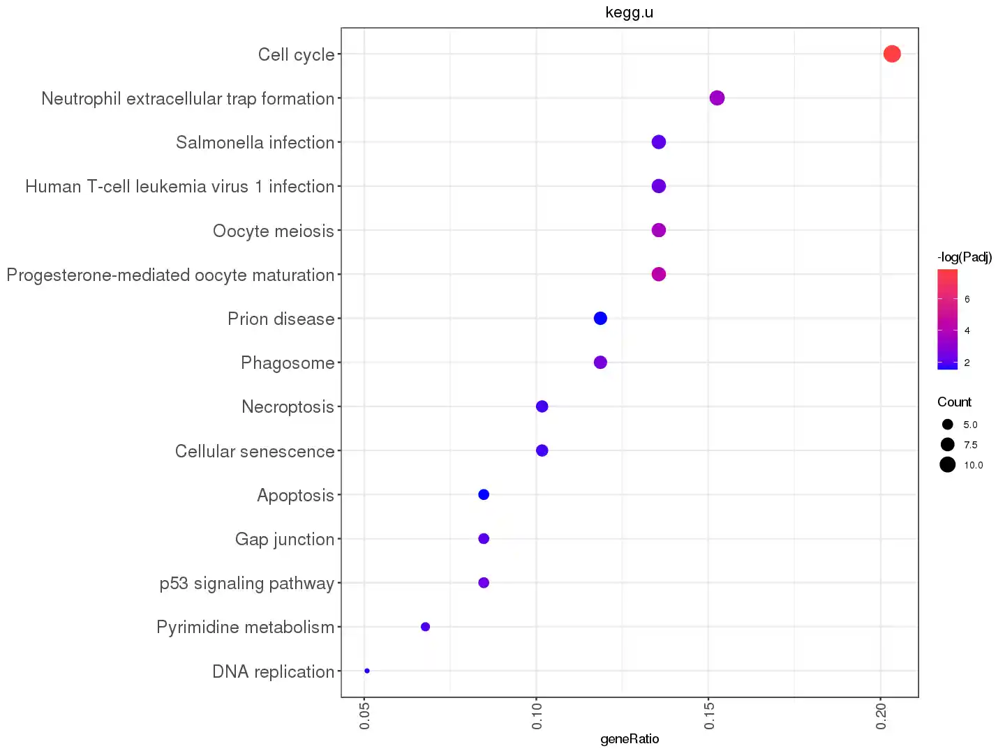
# clusterProfiler作kegg富集分析
library(clusterProfiler)
library(enrichplot)
library(forcats)

f_id2name_fuck <- function(lc_exp, lc_db){
    if(!is.data.frame(lc_db)){
        lc_ids <- toTable(lc_db)
    }else{
        lc_ids <- lc_db
    }
    res_n <- rownames(lc_exp)
    res_n <- res_n[res_n %in% lc_ids[[1]]]
    res <- lc_exp[res_n,]
    if(!is.data.frame(res)){res=data.frame(row.names = res_n, res)}
    lc_ids=lc_ids[match(rownames(res),lc_ids[[1]]),]
    lc_tmp = by(res,
         lc_ids[[2]],
         function(x) rownames(x)[which.max(rowMeans(x))])
    lc_probes = as.character(lc_tmp)
    res_n <- rownames(res)
    res_n <- res_n[res_n %in% lc_probes]
    res = res[res_n,]
    if(!is.data.frame(res)){res=data.frame(row.names = res_n, res)}  
    rownames(res)=lc_ids[match(rownames(res),lc_ids[[1]]),2]
    res
}

library(org.Hs.eg.db)
f_id2name_sb <- function(lc_cgene, keytype="SYMBOL", columns="ENTREZID"){
    res=select(org.Hs.eg.db,keys=lc_cgene,columns=columns, keytype=keytype)
    res <- subset(res, !is.na(ENTREZID))
    res$ENTREZID
}

library(ggplot2)
library(DOSE)
f_kegg_p <- function(keggr2, n = 15){
    keggr <- subset(keggr2@result, p.adjust < 0.05)
    keggr[['-log(Padj)']] <- -log10(keggr[['p.adjust']])
    keggr[['geneRatio']] <- parse_ratio(keggr[['GeneRatio']])
    keggr$Description <- factor(keggr$Description, 
                                       levels=keggr[order(keggr$geneRatio),]$Description)
    ggplot(head(keggr,n),aes(x=geneRatio,y=Description))+
        geom_point(aes(color=`-log(Padj)`,
                 size=`Count`))+
        theme_bw()+
        scale_color_gradient(low="blue1",high="brown1")+
        labs(y=NULL) + 
        theme(axis.text.x=element_text(angle=90,hjust = 1,vjust=0.5, size = 12),
             axis.text.y=element_text(size = 15))
}

ENTREZID=f_id2name_sb(rownames(scRNA))

kegg.u <- enrichKEGG(gene = f_id2name_sb(usignificant_markers$gene),
      organism = search_kegg_organism('Homo sapiens')$kegg_code,
      universe = ENTREZID,
      pAdjustMethod = "fdr",
      qvalueCutoff =0.05)

f_kegg_p(kegg.u, n =15) %>% f_title("kegg.u")
f_kegg_p(kegg.d, n =15) %>% f_title("kegg.d")

第三步 GO

GO.U.CC <- enrichGO(gene = f_id2name_sb(usignificant_markers$gene),
                    keyType = "ENTREZID",
                   OrgDb= 'org.Hs.eg.db',
                   ont = "CC",
                   universe = ENTREZID,
                   pAdjustMethod = "fdr",
                   qvalueCutoff = 0.05,
                   readable = TRUE)
GO.U.BP <- enrichGO(gene = f_id2name_sb(usignificant_markers$gene),
                    keyType = "ENTREZID",
                   OrgDb= 'org.Hs.eg.db',
                   ont = "BP",
                   universe = ENTREZID,
                   pAdjustMethod = "fdr",
                   qvalueCutoff = 0.05,
                   readable = TRUE)
GO.U.MF <- enrichGO(gene = f_id2name_sb(usignificant_markers$gene),
                    keyType = "ENTREZID",
                   OrgDb= 'org.Hs.eg.db',
                   ont = "MF",
                   universe = ENTREZID,
                   pAdjustMethod = "fdr",
                   qvalueCutoff = 0.05,
                   readable = TRUE)

f_kegg_p(GO.U.CC, n =15) %>% f_title("GO.U.CC")
f_kegg_p(GO.U.BP, n =15) %>% f_title("GO.U.BP")
f_kegg_p(GO.U.MF, n =15) %>% f_title("GO.U.MF")

第四步 GESA

f_gse_fuck <- function(geneSym, logFC, keytype="SYMBOL", columns="ENTREZID", lc_order=T){
    res=select(org.Hs.eg.db,keys=geneSym,columns=columns, keytype=keytype)
    res <- cbind(res, logFC)
    res <- subset(res, !is.na(ENTREZID))
    if(lc_order){res <- res[order(res$logFC, decreasing = T),]}
    res2 <- res$logFC
    if(lc_order){
        names(res2) <- res[[columns]]
    }else{
        names(res2) <- res[[keytype]]
    }
    res2
}

lgene <- f_gse_fuck(significant_markers$gene,significant_markers$avg_log2FC)

gsekegg <- gseKEGG(gene = lgene,
      organism = search_kegg_organism('Homo sapiens')$kegg_code,
      pAdjustMethod = "fdr")

GO.CC <- gseGO(gene = lgene,
                   keyType = "ENTREZID",
                   OrgDb= org.Hs.eg.db,
                   ont = "CC",
                   pAdjustMethod = "fdr")

GO.BP <- gseGO(gene = lgene,
                   keyType = "ENTREZID",
                   OrgDb= org.Hs.eg.db,
                   ont = "CC",
                   pAdjustMethod = "fdr")

options(repr.plot.width=9, repr.plot.height=9)
gseaplot2(gsekegg,geneSetID=head(which(gsekegg@result$enrichmentScore>0.4),15))
gseaplot2(gsekegg,geneSetID=head(which(gsekegg@result$enrichmentScore < -0.3),6))

gseaplot2(GO.CC,geneSetID=head(which(GO.CC@result$enrichmentScore>0.4),15))
gseaplot2(GO.CC,geneSetID=head(which(GO.CC@result$enrichmentScore < -0.3),6))

gseaplot2(GO.BP,geneSetID=head(which(GO.BP@result$enrichmentScore>0.4),15))
gseaplot2(GO.BP,geneSetID=head(which(GO.BP@result$enrichmentScore < -0.3),6))

第五步 GO terms关系网络图

# options(BioC_mirror="https://mirrors.tuna.tsinghua.edu.cn/bioconductor")
# BiocManager::install("ggnewscale")
library(enrichplot)

kegg.u2 <- pairwise_termsim(kegg.u)
emapplot(kegg.u2,showCategory=15) 

GO.U.MF2 <- pairwise_termsim(GO.U.MF)
emapplot(GO.U.MF2,showCategory=15) 

第六步 共同基因绘图

f_kegg_readable_1 <- function(Oj, columns="SYMBOL", keytype="ENTREZID"){
    ge <- Oj@gene
    ge <- select(org.Hs.eg.db,keys=ge,columns=columns, keytype=keytype)
    ge2sy <- ge[[columns]]
    names(ge2sy) <- ge[[keytype]]
    Oj@gene2Symbol <- ge2sy
    Oj
}
f_kegg_readable_2 <- function(str, ge2sy){
    res <- strsplit(str, '/')
    paste(unlist(ge2sy[unlist(res)]),sep = '', collapse="/")
}
f_kegg_readable <- function(Oj){
    res <- f_kegg_readable_1(Oj)
    kegg.u2@result$geneID <- lapply(kegg.u2@result$geneID, f_kegg_readable_2, Oj@gene2Symbol)
    kegg.u2
}

cnetplot(GO.U.BP2, foldChange= f_gse_fuck(usignificant_markers$gene,usignificant_markers$avg_log2FC, lc_order = F))
cnetplot(GO.U.MF2, foldChange= f_gse_fuck(usignificant_markers$gene,usignificant_markers$avg_log2FC, lc_order = F))

cnetplot(f_kegg_readable(kegg.u2), foldChange= f_gse_fuck(usignificant_markers$gene,usignificant_markers$avg_log2FC, lc_order = F))