1
2
3
4
5
6
7
8
9
10
11
12
13
14
15
16
17
18
19
20
21
| options(repr.plot.width=12, repr.plot.height=12)
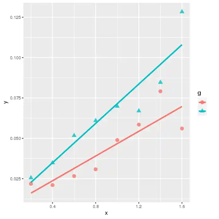
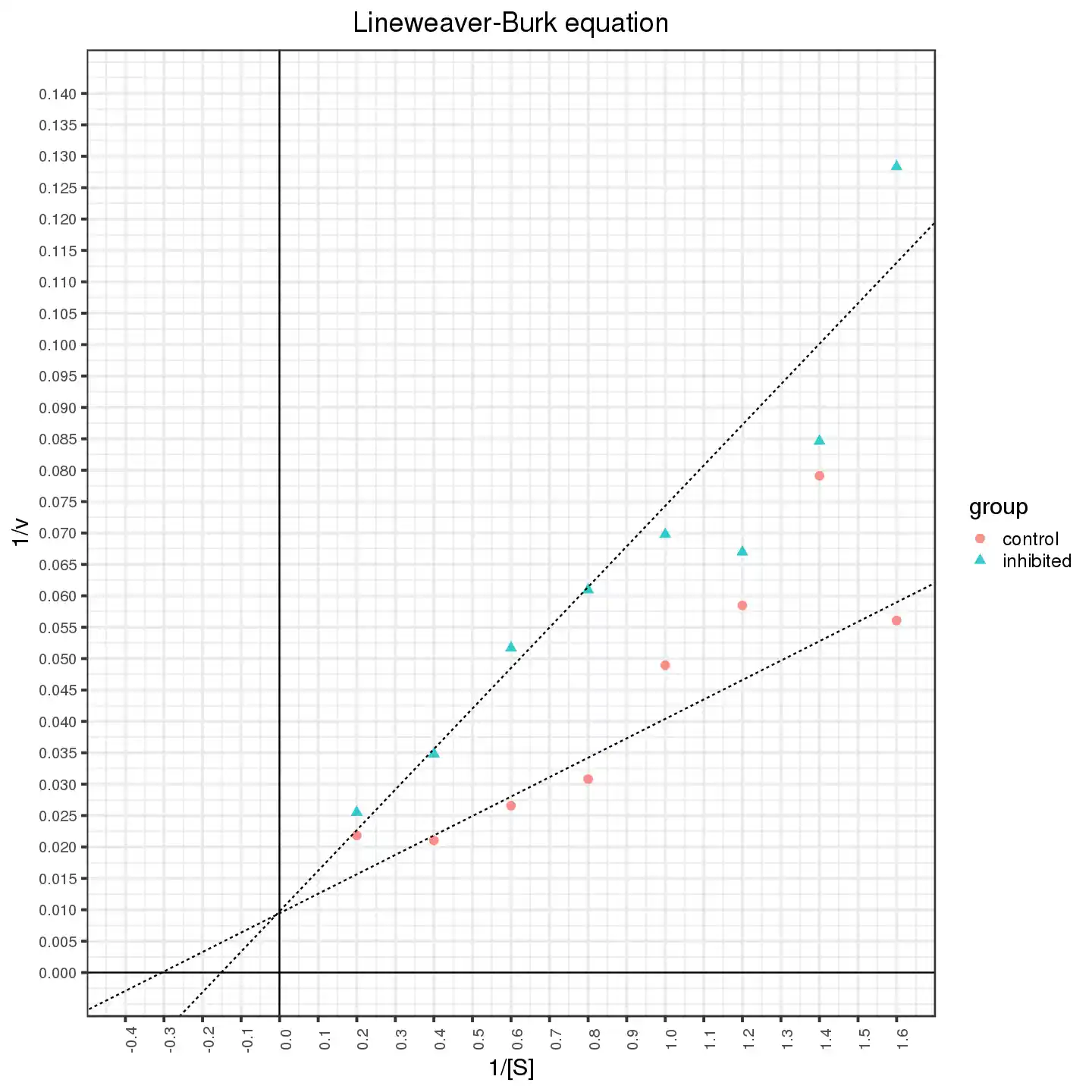
ggplot(data = f_gp_xyn(data),aes(x=x,y=y,colour = g, shape = g))+
geom_point(size=3,alpha=0.8) +
geom_abline(intercept = s3$coefficients[[1]], slope = s3$coefficients[[2]], linetype="dashed")+
geom_abline(intercept = s4$coefficients[[1]], slope = s4$coefficients[[2]], linetype="dashed")+
scale_x_continuous(limits = c(-0.4,1.6), breaks=seq(-0.4, 1.6, 0.1))+
scale_y_continuous(limits = c(0,0.14), breaks=seq(0, 0.14, 0.005))+
labs (title="Lineweaver-Burk equation",x="1/[S]",y="1/v")+
theme_light() +
theme_bw(base_size=18) +
theme(plot.title = element_text(hjust = 0.5),
axis.text.y = element_text(size = 12),
axis.text.x = element_text(size = 12, angle=90))+
geom_hline(aes(yintercept=0))+geom_vline(aes(xintercept=0))+
scale_shape_discrete(name="group",
labels=c("control", "inhibited"))+
scale_color_discrete(name="group",
labels=c("control", "inhibited"))
ggsave("example2.pdf")
|