评价临床预测模型

模型来源参考1参考2

安装补充包

1
2
3
4
library(pROC) #绘制ROC曲线
library(timeROC)
library(ggDCA) #绘制DCA曲线
library(nricens) #计算NRI值

Logistic回归的诺莫图的校准图

1
2
3
4
5
6
fit <- lrm(formula(lrmf), data=df, x=TRUE, y=TRUE, maxit=1000)
cal <- calibrate(fit, method="boot", B=1000)
plot(cal,
  xlab="Nomogram-predicted probability of nonadherence",
  ylab="Actual diagnosed nonadherence (proportion)",
  sub=F)

其中Bias-corrected为校正曲线,而对角线Ideal为理想的曲线。校正曲线与理想曲线之间越相近,说明模型的预测能力越好。

COX回归的诺莫图的校准图

1
2
3
4
5
6
7
8
9
10
11
12
f_cph_2 <- cph(formula(coxmf),
x=T, y=T, surv=T,
data=df)
cal_2 <- calibrate(f_cph_2, u=5, cmethod='KM', m=15, B=200)# usually B=200 or 300, u=5表示五年
options(repr.plot.width=10, repr.plot.height=10)
plot(cal_2,lwd=2,lty=1, ##设置线条宽度和线条类型
errbar.col=c(rgb(0,118,192,maxColorValue = 255)), ##设置一个颜色
xlab='Nomogram-Predicted Probability of 5 years DFS',#便签
ylab='Actual 5 years DFS(proportion)',#标签
col=c(rgb(192,98,83,maxColorValue = 255)),#设置一个颜色
xlim = c(0,1),ylim = c(0,1),##x轴和y轴范围
mgp = c(2, 1, 0)) #控制坐标轴的位置

计算C指数

  • rcorrcens((dcf_status==0)~predict(f2), data = df)
  • <0.5 模型没有任何预测能力
  • 0.51-0.7 较差的准确性
  • 0.71-0.9 中等的准确性
  • > 0.9 高度的准确性

ROC曲线

1
2
3
4
5
6
7
8
9
10
gfit <- roc((dcf_status==0)~predict(f2), data = df)
options(repr.plot.width=6, repr.plot.height=6)
plot(gfit,
  print.auc=TRUE, #输出AUC值
  print.thres=TRUE, #输出cut-off值
  main = "ROC CURVE", #设置图形的标题
  col= "red", #曲线颜色
  print.thres.col="black", #cut-off值字体的颜色
  identity.col="blue", #对角线颜色
  identity.lty=1,identity.lwd=1)
  • AUC值为 0.656
  • 0.5~0.7 模型的效果较低
  • 0.7~0.85 效果一般
  • 0.85~0.95 效果很好
  • 最佳截断值cut 2.898
  • 当以2.898进行分组时,两组之间具有最佳的区分度

Logistic回归的DCA曲线

1
2
3
4
5
6
7
8
9
10
11
12
library(rmda) #绘制DCA曲线
modul<- decision_curve(data= df,
  formula(lrmf),
  family = binomial(link ='logit'),
  thresholds= seq(0,1, by = 0.01),
  confidence.intervals = 0.95)
plot_decision_curve(modul,
  curve.names="Nonadherence prediction nomogram", #曲线名称
  xlab="Threshold probability", #x轴名称
  cost.benefit.axis =FALSE, col= "blue",
  confidence.intervals=FALSE,
  standardize = FALSE)

COX回归的DCA曲线

1
2
3
4
5
6
7
8
9
10
11
12
13
14
15
16
library(car)
library(rms)
library(pROC)
library(timeROC)
library(ggDCA)
df <- readRDS('Cox_df.rds')
df[,'dcf_status'] = ifelse(df[,'dcf_status']==0,1,2)
dd=datadist(df)
options(datadist="dd")
coxmf <- paste0("Surv(dcf_time, dcf_status)~", paste(colnames(df)[1:10], collapse = '+'))
coxmf
f_cph_2 <- cph(formula(coxmf),
x=T, y=T, surv=T,
data=df)
dca_training <- dca(f_cph_2, times=c(5*365, 10*365)) #五年、十年
ggplot(dca_training)

Logistic回归的NRI指数

1
2
3
4
5
6
7
8
9
10
11
12
13
14
15
16
17
18
19
20
lrmf_a <- paste0("factor(dcf_status)~", paste(colnames(df)[1:9], collapse = '+'))
lrmf_b <- paste0("factor(dcf_status)~", paste(colnames(df)[1:10], collapse = '+'))
fit_A <- glm(formula(lrmf_a), data = df, family = binomial(link="logit"), x=TRUE)
fit_B <- glm(formula(lrmf_b), data = df, family = binomial(link="logit"), x=TRUE)
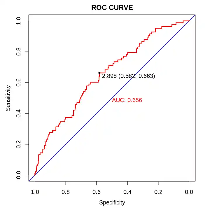
gfit <- roc(factor(dcf_status)~predict(fit_A), data = df)
options(repr.plot.width=10, repr.plot.height=10)
plot(gfit,
  print.auc=TRUE, #输出AUC值
  print.thres=TRUE, #输出cut-off值
  main = "ROC CURVE", #设置图形的标题
  col= "red", #曲线颜色
  print.thres.col="black", #cut-off值字体的颜色
  identity.col="blue", #对角线颜色
  identity.lty=1,identity.lwd=1)
NRI <- nribin(mdl.std = fit_A, mdl.new = fit_B,
  updown = 'diff',
  cut = 0.05, niter = 500, alpha = 0.05)
NRI <- nribin(mdl.std = fit_A, mdl.new = fit_B,
  updown = 'category',
  cut = 1.791, niter = 500, alpha = 0.05)

根据之前模型的ROC分析确定的切点cut,之后的分析见爱科学


评价临床预测模型
https://b.limour.top/1915.html
Author
Limour
Posted on
July 17, 2022
Licensed under