COXPH绘制ROC曲线

安装补充包

• conda activate ggsurvplot
• # conda install -c conda-forge r-pec -y
• conda install -c conda-forge r-survivalroc -y
• # conda install -c conda-forge r-ggsci -y
• # conda install -c conda-forge r-scales -y
• install.packages(‘nomogramFormula’)

整理数据

library(survival)
clinical <- readRDS('../A_ref_A_fiig.3_A_B/clinical.rds')
table(clinical$PSA)
clinical <- clinical[0 < clinical$PSA & clinical$PSA<40,]
clinical$PSA <- log(clinical$PSA)
dat <- readRDS('../../../COXPH/data/PRAD.rds')
dat$meta <- dat$meta[rownames(clinical),]
y <- Surv(round(dat$meta$pfs_time,2), dat$meta$pfs_status == 1)
y <- data.matrix(y)
df <- cbind(clinical, y)
table(df$T)
df$T2vs3 <- 0
df$T2vs3[!(df$T %in% c('T2a', 'T2b', 'T2c'))] <- 1
table(df$N)
df$N0vs1 <- 0
df$N0vs1[!(df$N == 'N0')] <- 1
df
saveRDS(df,'clinical.rds')
coxmf <- paste0("Surv(time, status==1)~PSA+Age+T2vs3+N0vs1+GS")
coxmf

计算C-index

res.cox <- coxph(formula(coxmf), data =  df)
tmp_res <- summary(res.cox)
Ci <- tmp_res$concordance['C']
Ci_se <- tmp_res$concordance['se(C)']
c(Ci-1.96*Ci_se,Ci+1.96*Ci_se)

基于survivalROC绘制ROC曲线

预测生存概率

library(car)
library(rms)
library(pROC)
library(timeROC)
library(ggDCA)
library(survivalROC)
library(pec)
f2 <- cph(formula(coxmf), data=df, x=T, y=T, surv = T) # 构建COX比例风险模型
df$`1-year` <- predictSurvProb(f2,newdata=df,times=1*12)
df$`3-year` <- predictSurvProb(f2,newdata=df,times=3*12)
df$`5-year` <- predictSurvProb(f2,newdata=df,times=5*12)
df

计算ROC曲线

# year1 <- survivalROC(Stime=df$time,##生存时间
#                      status=df$status,## 终止事件
#                      marker=df$`1-year`, ## marker value    
#                      predict.time = 1*12,## 预测时间截点
#                      span = 0.25*nobs^(-0.20))##span,NNE法的namda
year1 <- survivalROC(Stime=df$time,##生存时间
                     status=df$status,## 终止事件
                     marker=-df$`1-year`, ## marker value    
                     predict.time = 1*12,## 预测时间截点
                     method="KM")
year3 <- survivalROC(Stime=df$time,##生存时间
                     status=df$status,## 终止事件
                     marker=-df$`3-year`, ## marker value    
                     predict.time = 3*12,## 预测时间截点
                     method="KM")
year5 <- survivalROC(Stime=df$time,##生存时间
                     status=df$status,## 终止事件
                     marker=-df$`5-year`, ## marker value    
                     predict.time = 5*12,## 预测时间截点
                     method="KM")

绘制ROC曲线

require(ggsci)
library("scales")
pal_nejm("default")(8)
show_col(pal_nejm("default")(8)) #挑选配色
 
options(repr.plot.width=8, repr.plot.height=8)
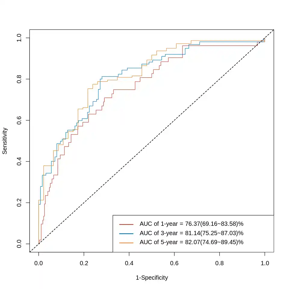
plot(year1$FP, year1$TP, ## x=FP,y=TP
     type="l",col="#BC3C29FF", ##线条设置
     xlim=c(0,1), ylim=c(0,1),   
     xlab=("FP"), ##连接
     ylab="TP",
     main="Time dependent ROC")## \n换行符
abline(0,1,col="gray",lty=2)##线条颜色
lines(year3$FP, year3$TP, type="l",col="#0072B5FF",xlim=c(0,1), ylim=c(0,1))
lines(year5$FP, year5$TP, type="l",col="#E18727FF",xlim=c(0,1), ylim=c(0,1))
 
legend(0.6,0.2,c(paste("AUC of 1-year =",round(year1$AUC,3)),
                 paste("AUC of 3-year =",round(year3$AUC,3)),
                 paste("AUC of 5-year =",round(year5$AUC,3))),
                 x.intersp=1, y.intersp=0.8,
                 lty= 1 ,lwd= 2,col=c("#BC3C29FF","#0072B5FF", "#E18727FF"),
                 bty = "n",# bty框的类型
                 seg.len=1,cex=0.8)# 

基于timeROC绘制ROC曲线

预测风险得分（前面先预测生存概率）

library(nomogramFormula)
surv <- Survival(f2) # 构建生存概率函数
dd=datadist(df)
options(datadist="dd") 
nom <- nomogram(f2, fun=list(function(x) {surv(1*12, x)},
                            function(x) {surv(3*12, x)},
                            function(x) {surv(5*12, x)}),
                             funlabel=c("1-year Disease-free Probability",
                                        "3-year Disease-free Probability",
                                        "5-year Disease-free Probability"))
 
options(repr.plot.width=12, repr.plot.height=6)
plot(nom, xfrac=.2)

results <- formula_rd(nomogram = nom)
df$points <- points_cal(formula = results$formula,rd=df)
df

计算ROC曲线

# years <- timeROC(T=df$time,delta=df$status,
#                   marker=df$points,cause=1,
#                   weighting="cox",
# #                   other_markers=as.matrix(df$`1-year`),
#                   times=12*c(1,3,5), ROC=T)
years <- timeROC(T=df$time,delta=df$status,
                      marker=df$points,cause=1,
                      weighting="marginal",
    #                   other_markers=as.matrix(df$`1-year`),
                      times=12*c(1,3,5), ROC=T, iid=T)
years

构造AUC描述

auc.ci <- confint(years, parm=NULL, level = 0.95,n.sim=2000)
auc.ci <- auc.ci$CI_AUC
auc.ci
 
years.auc1 <- paste0(round(years$AUC[1],4)*100,'(',auc.ci[1,1],'~',auc.ci[1,2],')%')
years.auc2 <- paste0(round(years$AUC[2],4)*100,'(',auc.ci[2,1],'~',auc.ci[2,2],')%')
years.auc3 <- paste0(round(years$AUC[3],4)*100,'(',auc.ci[3,1],'~',auc.ci[3,2],')%')

绘制ROC曲线

options(repr.plot.width=8, repr.plot.height=8)
plot(years,time=12*1,title="Time dependent ROC",col="#BC3C29FF")        
plot(years,time=12*3,add=TRUE,col="#0072B5FF") 
plot(years,time=12*5,add=TRUE,col="#E18727FF") 
legend("bottomright",c(paste("AUC of 1-year =",years.auc1),
                 paste("AUC of 3-year =",years.auc2),
                 paste("AUC of 5-year =",years.auc3)),
       col=c("#BC3C29FF","#0072B5FF","#E18727FF"),lty=1,lwd=2)

对两个模型的ROC曲线进行检验

compare(model1_years,model2years,adjusted=T)