1
2
3
4
5
6
7
8
9
10
11
12
13
14
15
16
17
18
19
20
21
22
23
24
25
26
27
28
29
30
31
32
33
34
35
36
37
38
39
40
41
42
43
44
45
46
47
48
49
50
51
52
53
54
55
56
57
58
59
60
61
62
63
64
65
66
67
68
69
70
71
72
73
74
75
76
77
78
79
80
81
82
83
84
85
86
87
88
89
90
91
92
93
94
95
96
97
98
99
100
101
102
103
104
105
106
107
108
109
110
111
112
113
114
115
116
117
118
119
120
121
122
| # 4、构造图片保存方法
f_image_output <- function(fileName, image, width=1920, height=1080, lc_pdf=T, lc_resolution=72){
if(lc_pdf){
width = width / lc_resolution
height = height / lc_resolution
pdf(paste(fileName, ".pdf", sep=""), width = width, height = height)
}else{
png(paste(fileName, ".png", sep=""), width = width, height = height)
}
print(image)
dev.off()
}
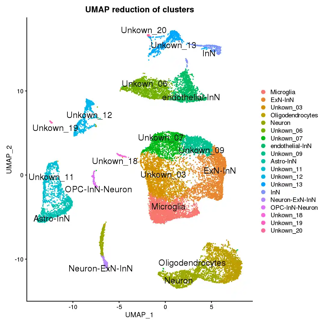
# 14、划分细胞群
scRNA <- FindNeighbors(scRNA, dims = 1:pca_dim)
scRNA <- FindClusters(scRNA, resolution = 0.5)
DimPlot(scRNA, reduction = lc_reduction)
# 16、寻找显著基因
all_markers <- FindAllMarkers(scRNA, only.pos = TRUE, min.pct = 0.25, logfc.threshold = 0.25)
significant_markers <- subset(all_markers, subset = p_val_adj<0.05)
write.csv(significant_markers, "significant_markers.csv")
f_cluster_averages <- function(lc_scRNA){
# 切分出Clusters
lc_clusters <- SplitObject(lc_scRNA, split.by = 'ident')
for (lc_i in 1:length(lc_clusters)){
lc_clusters[[lc_i]] <- lc_clusters[[lc_i]][[lc_clusters[[lc_i]]@active.assay]]@scale.data
}
for (lc_i in 1:length(lc_clusters)){
lc_clusters[[lc_i]] <- apply(lc_clusters[[lc_i]],1,mean)
}
lc_clusters <- data.frame(lc_clusters)
scale(lc_clusters)
}
library(Hmisc)
library(corrplot)
f_corrplot <- function(lc_scdata){
lc_cor <- rcorr(lc_scdata)
lc_cor$P[is.na(lc_cor$P)]=0
lc_cor$P <- -log10(lc_cor$P)
lc_cor$P[is.infinite(lc_cor$P)] = max(lc_cor$P[!is.infinite(lc_cor$P)]) + 1
corrplot(lc_cor$r, type="upper",tl.pos = "d",order = "AOE", p.mat = lc_cor$P, insig = "p-value")
corrplot(lc_cor$r, add=TRUE, type="lower", method="number",order = "AOE", diag=FALSE,tl.pos="n", cl.pos="n")
}
# 3、准备好新的marker genes list
gl_MarkerGene <- read.csv(file.path(root_path, "cellType_Markers.csv"), header = F)
colnames(gl_MarkerGene) <- c('marker','celltype')
gl_Markers_ExN <- read.table(file.path(root_path, "ExN.csv"), header = F)
colnames(gl_Markers_ExN) <- c('marker','celltype')
gl_Markers_InN <- read.table(file.path(root_path, "InN.csv"), header = F)
colnames(gl_Markers_InN) <- c('marker','celltype')
gl_TS3 <- read.csv(file.path(root_path, "TableS3.csv"))
colnames(gl_TS3) <- c('marker','celltype')
gl_TS3$celltype <- substr(gl_TS3$celltype,1,3)
f_setRowName <- function(lc_df, lc_colName){
lc_df <- lc_df[order(lc_df[[lc_colName]]),]
tp_index <- duplicated(lc_df[[lc_colName]])
lc_df <- lc_df[!tp_index,]
rownames(lc_df) <- lc_df[[lc_colName]]
lc_df
}
gl_MarkerGene <- f_setRowName(gl_MarkerGene, 'marker')
gl_TS3 <- f_setRowName(gl_TS3, 'marker')
gl_Markers_ExN <- f_setRowName(gl_Markers_ExN, 'marker')
gl_Markers_InN <- f_setRowName(gl_Markers_InN, 'marker')
# 18、绘制已知基因在不同cluster内的Violin plots
# 18.1 定义Violin plots绘制方法
f_get_cell_markers <- function(lc_cellType, lc_significant_markers, lc_MarkerGene){
lc_features <- rownames(subset(lc_MarkerGene, subset = celltype == lc_cellType))
lc_features <- lc_features[lc_features %in% lc_significant_markers$gene]
lc_features
}
f_VlnPlot <- function(sObject, lc_cellType, lc_significant_markers, lc_MarkerGene) {
lc_features <- f_get_cell_markers(lc_cellType, lc_significant_markers, lc_MarkerGene)
if (length(lc_features)!=0){VlnPlot(sObject, features = lc_features)}
else{ F }
}
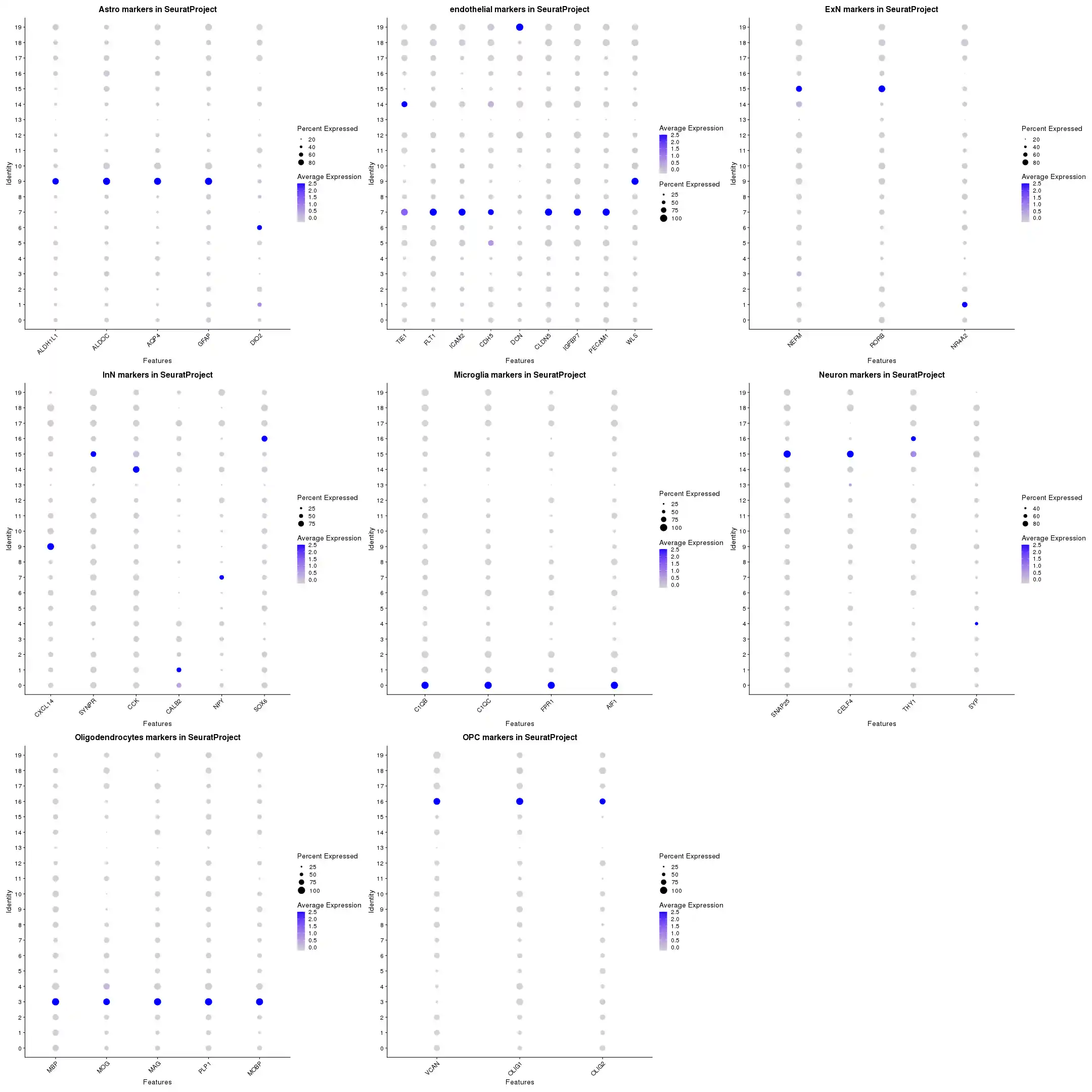
f_get_m_p <- function(sObject, lc_cellType, lc_significant_markers, lc_MarkerGene){
lc_features <- f_get_cell_markers(lc_cellType, lc_significant_markers, lc_MarkerGene)
if (length(lc_features)==0){return(NULL)}
DotPlot(sObject, features = lc_features) + RotatedAxis() +
ggtitle(sprintf("%s markers in %s", lc_cellType, sObject@project.name)) +
theme(plot.title = element_text(hjust = 0.5))
}
# 18.2 绘制已知细胞类型的marker genes在本数据集中的pattern
f_get_all_celltype <- function(lc_MarkerGene){
tp_cellTypes <- lc_MarkerGene$celltype # 获取所有细胞类型
tp_cellTypes <- sort(tp_cellTypes) # 排序
tp_cellTypes <- tp_cellTypes[!duplicated(tp_cellTypes)] #去重
tp_cellTypes
}
f_get_m_p_a <- function(sObject, lc_significant_markers, lc_MarkerGene){
lc_cellTypes <- f_get_all_celltype(lc_MarkerGene)
tp_emm <- 2
for (lc_j in 1:length(lc_cellTypes)){
lc_image <- f_get_m_p(sObject, lc_cellTypes[lc_j], lc_significant_markers, lc_MarkerGene)
if (!is.null(lc_image)){ break }
tp_emm <- tp_emm + 1
}
if (tp_emm > length(lc_cellTypes)){return(NULL)}
for(lc_j in tp_emm:length(lc_cellTypes)){
lc_image <- lc_image + f_get_m_p(sObject, lc_cellTypes[[lc_j]], lc_significant_markers, lc_MarkerGene)
}
lc_image <- lc_image + plot_layout(ncol = 3)
lc_image
}
tp_image <- f_get_m_p_a(scRNA, significant_markers, gl_MarkerGene)
f_image_output('gl_MarkerGene',tp_image, width = 2160, height = 2160)
|