SingleR (六) 切出指定群并检验

第一步 切出神经细胞

1
2
3
4
5
6
7
8
9
10
11
12
13
14
15
16
17
18
19
20
21
22
23
24
25
26
27
28
29
30
31
32
33
34
35
36
37
38
39
40
41
42
43
44
45
46
47
48
49
50
51
52
53
54
55
56
57
58
59
60
61
62
63
64
65
66
67
68
69
70
71
72
73
74
75
76
77
78
79
80
81
82
83
84
85
86
87
88
89
90
91
92
93
94
95
96
97
98
99
100
101
102
103
104
105
106
107
108
109
110
111
112
113
114
115
116
117
118
119
120
121
122
123
124
125
126
127
128
129
130
131
132
133
library(Matrix)
library(Seurat)
library(plyr)
library(dplyr)
library(patchwork)
library(purrr)

library(RColorBrewer)
library(ggplot2)
library(ggrepel)
blank_theme <- theme_minimal()+
theme(
axis.title.x = element_blank(),
axis.text.x=element_blank(),
axis.title.y = element_blank(),
axis.text.y=element_blank(),
panel.border = element_blank(),
panel.grid=element_blank(),
axis.ticks = element_blank(),
plot.title=element_text(size=14, face="bold",hjust = 0.5)
)
col_Paired <- colorRampPalette(brewer.pal(12, "Paired"))
f_pie <- function(lc_x, lc_main, lc_x_p = 1.3, lc_r = T){
lc_cols <- col_Paired(length(lc_x))
lc_v <- as.vector(100*lc_x)
lc_df <- data.frame(type = names(lc_x), nums = lc_v)
lc_df <- lc_df[order(lc_df$type),]
lc_percent = sprintf('%0.2f%%',lc_df$nums)
if(lc_r){
lc_df$pos <- with(lc_df, 100-cumsum(nums)+nums/2)
}else{
lc_df$pos <- with(lc_df, cumsum(nums)-nums/2)
}
lc_pie <- ggplot(data = lc_df, mapping = aes(x = 1, y = nums, fill = type)) + geom_bar(stat = 'identity')
# print(lc_df)
# print(lc_pie)
lc_pie <- lc_pie + coord_polar("y", start=0, direction = 1) + scale_fill_manual(values=lc_cols) + blank_theme
lc_pie <- lc_pie + geom_text_repel(aes(x = lc_x_p, y=pos),label= lc_percent, force = T,
arrow = arrow(length=unit(0.01, "npc")), segment.color = "#cccccc", segment.size = 0.5)
lc_pie <- lc_pie + labs(title = lc_main)
lc_pie
}

# 配置数据和mark基因表的路径
root_path = "~/zlliu/R_data/hBLA"

# 配置结果保存路径
output_path = "~/zlliu/R_data/21.10.01.10x"
if (!file.exists(output_path)){dir.create(output_path)}

# 设置工作目录,输出文件将保存在此目录下
setwd(output_path)
getwd()

scRNA <- readRDS('~/zlliu/R_data/21.09.29.10x/scRNA.rds')

scRNA

f_UMAP_more <- function(sObject, lc_group.by, lc_reduction="umap"){
res <- (DimPlot(sObject, reduction = lc_reduction, group.by = lc_group.by[1], label = T, repel = T, label.size = 6) +
labs(title = lc_group.by[1]))
for(lc_i in 2:length(lc_group.by)){
res <- res/
(DimPlot(sObject, reduction = lc_reduction, group.by = lc_group.by[lc_i], label = T, repel = T, label.size = 6) +
labs(title = lc_group.by[lc_i]))
}
res
}

scRNA@meta.data

Idents(scRNA) <- scRNA[["hM1_hmca_class"]]

options(repr.plot.width=9, repr.plot.height=18)
options(ggrepel.max.overlaps = Inf)
f_UMAP_more(scRNA, c('hM1_hmca_class', 'hM1_class', 'hmca_class'))

levels(scRNA)

unique(scRNA[["hmca_class"]])

unique(scRNA[["hM1_class"]])

n_ExN <- c('L4 IT','L5 IT','L5 ET','IT','L6b','L5/6 IT Car3','L6 IT','L2/3 IT','L5/6 NP','L6 IT Car3','L6 CT')

n_InN <- c('Lamp5','Pvalb','Sst','Vip','Sncg')

n_NoN <- c('Astro','PAX6','Endo','Micro-PVM','OPC','Oligo','Pericyte','VLMC')

n_groups <- list(NoN=n_NoN, ExN=n_ExN, InN=n_InN)

f_listUpdateRe <- function(lc_obj, lc_bool, lc_item){
lc_obj[lc_bool] <- rep(lc_item,times=sum(lc_bool))
lc_obj
}

f_grouplabel <- function(lc_meta.data, lc_groups){
res <- lc_meta.data[[1]]
for(lc_g in names(lc_groups)){
lc_bool = (res %in% lc_groups[[lc_g]])
for(c_n in colnames(lc_meta.data)){
lc_bool = lc_bool (lc_meta.data[[c_n]] %in% lc_groups[[lc_g]])
}
res <- f_listUpdateRe(res, lc_bool, lc_g)
}
names(res) <- rownames(lc_meta.data)
res
}

scRNA[['n_groups']] <- f_grouplabel(scRNA[[c("hM1_hmca_class","hM1_class","hmca_class")]], n_groups)

options(repr.plot.width=9, repr.plot.height=12)
options(ggrepel.max.overlaps = Inf)
f_UMAP_more(scRNA, c('hM1_hmca_class', 'n_groups'))

sc_Neuron <- subset(x = scRNA, n_groups %in% c("InN", "ExN"))
saveRDS(sc_Neuron, "sc_Neuron.rds")

f_UMAP_more(sc_Neuron, c('hM1_hmca_class', 'hM1_class', 'hmca_class'))

scRNA[['hM1_hmca_groups']] <- f_grouplabel(scRNA[["hM1_hmca_class"]], n_groups)
scRNA[['hmca_groups']] <- f_grouplabel(scRNA[["hmca_class"]], n_groups)
scRNA[['hM1_groups']] <- f_grouplabel(scRNA[["hM1_class"]], n_groups)

sc_Neuron <- subset(x = scRNA, hmca_groups %in% c("InN", "ExN"))
saveRDS(sc_Neuron, "sc_Neuron.rds")
Idents(sc_Neuron) <- sc_Neuron[['hmca_class']]

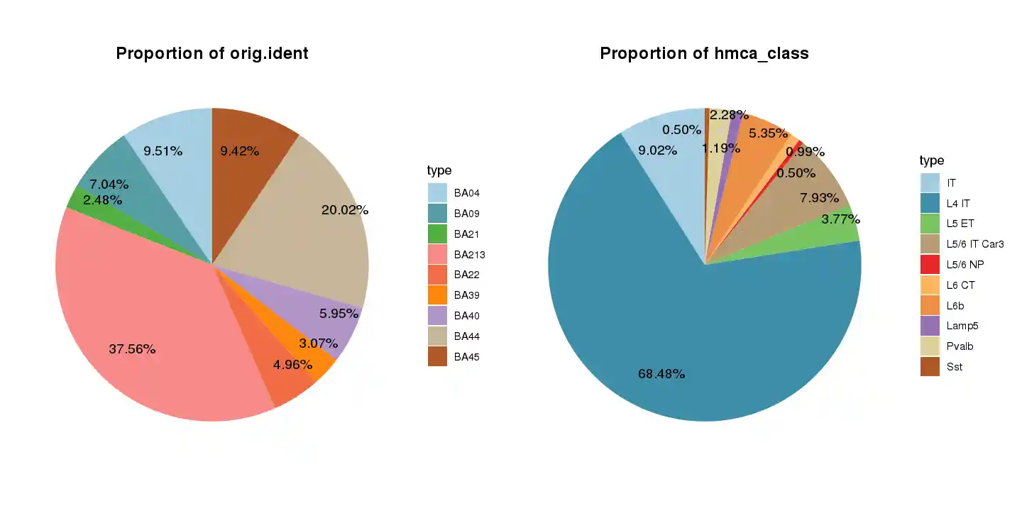
f_pie_metaN <- function(sObject, lc_group.by){
tp_data <- prop.table(table(sObject[[lc_group.by]]))
f_pie(tp_data, sprintf('Proportion of %s', lc_group.by))
}

第二步 画图查看相关性

1
2
3
4
5
6
7
8
9
10
11
12
13
14
15
16
17
18
19
20
21
22
23
24
25
26
27
28
29
30
31
32
33
34
35
f_cluster_averages <- function(lc_scRNA){
# 切分出Clusters
lc_clusters <- SplitObject(lc_scRNA, split.by = 'ident')
for (lc_i in 1:length(lc_clusters)){
lc_clusters[[lc_i]] <- lc_clusters[[lc_i]][[lc_clusters[[lc_i]]@active.assay]]@scale.data
}
for (lc_i in 1:length(lc_clusters)){
lc_clusters[[lc_i]] <- apply(lc_clusters[[lc_i]],1,mean)
}
lc_clusters <- data.frame(lc_clusters)
scale(lc_clusters)
}

library(Hmisc)
library(corrplot)
f_corrplot <- function(lc_scdata){
lc_cor <- rcorr(lc_scdata)
lc_cor$P[is.na(lc_cor$P)]=0
lc_cor$P <- -log10(lc_cor$P)
lc_cor$P[is.infinite(lc_cor$P)] = max(lc_cor$P[!is.infinite(lc_cor$P)]) + 1
corrplot(lc_cor$r, type="upper",tl.pos = "t", order = "hclust",
p.mat = lc_cor$P, insig = "p-value")
corrplot(lc_cor$r, add=TRUE, type="lower", method="number",col="black",
order = "hclust", tl.pos="l", cl.pos="n",addCoefasPercent = T)
}
tp_d <- f_cluster_averages(sc_Neuron)

library(Hmisc)
library(ggcorrplot)
f_corrplot <- function(lc_scdata){
lc_cor <- rcorr(lc_scdata)
lc_cor$P[is.na(lc_cor$P)]=0
ggcorrplot(lc_cor$r, type="full",hc.order = T, lab = T, p.mat = lc_cor$P)
}

第三步 Cluster差异基因

1
2
3
4
5
6
7
8
9
10
11
12
13
14
15
16
17
18
19
20
21
22
23
24
25
26
27
28
29
30
31
32
33
34
35
36
37
38
39
40
41
42
43
44
45
46
47
48
49
50
51
52
53
54
55
56
57
58
59
60
61
62
63
64
65
66
67
68
69
70
71
72
73
74
75
76
77
78
79
80
81
82
Idents(sc_Neuron) <- sc_Neuron[['hmca_class']]
all_markers <- FindAllMarkers(sc_Neuron, only.pos = TRUE, min.pct = 0.25, logfc.threshold = 0.25)
significant_markers <- subset(all_markers, subset = p_val_adj<0.05)
write.csv(significant_markers, "significant_markers.csv")

significant_markers %>%
group_by(cluster) %>%
top_n(n = 10, wt = avg_log2FC) -> top10
DoHeatmap(sc_Neuron, features = top10$gene)

gl_Markers_ExN <- read.table(file.path(root_path, "ExN.csv"), header = F)
colnames(gl_Markers_ExN) <- c('marker','celltype')

gl_Markers_InN <- read.table(file.path(root_path, "InN.csv"), header = F)
colnames(gl_Markers_InN) <- c('marker','celltype')

f_setRowName <- function(lc_df, lc_colName){
lc_df <- lc_df[order(lc_df[[lc_colName]]),]
tp_index <- duplicated(lc_df[[lc_colName]])
lc_df <- lc_df[!tp_index,]
rownames(lc_df) <- lc_df[[lc_colName]]
lc_df
}

gl_Markers_ExN <- f_setRowName(gl_Markers_ExN, 'marker')
gl_Markers_InN <- f_setRowName(gl_Markers_InN, 'marker')

gl_ExN_InN <- rbind(gl_Markers_ExN, gl_Markers_InN)

# 18、绘制已知基因在不同cluster内的Violin plots
# 18.1 定义Violin plots绘制方法
f_get_cell_markers <- function(lc_cellType, lc_significant_markers, lc_MarkerGene){
lc_features <- rownames(subset(lc_MarkerGene, subset = celltype == lc_cellType))
lc_features <- lc_features[lc_features %in% lc_significant_markers$gene]
lc_features
}
f_VlnPlot <- function(sObject, lc_cellType, lc_significant_markers, lc_MarkerGene) {
lc_features <- f_get_cell_markers(lc_cellType, lc_significant_markers, lc_MarkerGene)
if (length(lc_features)!=0){VlnPlot(sObject, features = lc_features)}
else{ F }
}

f_get_m_p <- function(sObject, lc_cellType, lc_significant_markers, lc_MarkerGene){
lc_features <- f_get_cell_markers(lc_cellType, lc_significant_markers, lc_MarkerGene)
if (length(lc_features)==0){return(NULL)}
DotPlot(sObject, features = lc_features) + RotatedAxis() +
ggtitle(sprintf("%s markers in %s", lc_cellType, sObject@project.name)) +
theme(plot.title = element_text(hjust = 0.5))
}

# 18.2 绘制已知细胞类型的marker genes在本数据集中的pattern
f_get_all_celltype <- function(lc_MarkerGene){
tp_cellTypes <- lc_MarkerGene$celltype # 获取所有细胞类型
tp_cellTypes <- sort(tp_cellTypes) # 排序
tp_cellTypes <- tp_cellTypes[!duplicated(tp_cellTypes)] #去重
tp_cellTypes
}

f_get_m_p_a <- function(sObject, lc_significant_markers, lc_MarkerGene){
lc_cellTypes <- f_get_all_celltype(lc_MarkerGene)
tp_emm <- 2
for (lc_j in 1:length(lc_cellTypes)){
lc_image <- f_get_m_p(sObject, lc_cellTypes[lc_j], lc_significant_markers, lc_MarkerGene)
if (!is.null(lc_image)){ break }
tp_emm <- tp_emm + 1
}

if (tp_emm > length(lc_cellTypes)){return(NULL)}

for(lc_j in tp_emm:length(lc_cellTypes)){
lc_image <- lc_image + f_get_m_p(sObject, lc_cellTypes[[lc_j]], lc_significant_markers, lc_MarkerGene)
}
lc_image <- lc_image + plot_layout(ncol = 3)
lc_image
}

f_image_output <- function(fileName, image, width=1920, height=1080){
png(paste(fileName, ".png", sep=""), width = width, height = height)
print(image)
dev.off()
}


SingleR (六) 切出指定群并检验
https://b.limour.top/829.html
Author
Limour
Posted on
October 1, 2021
Licensed under